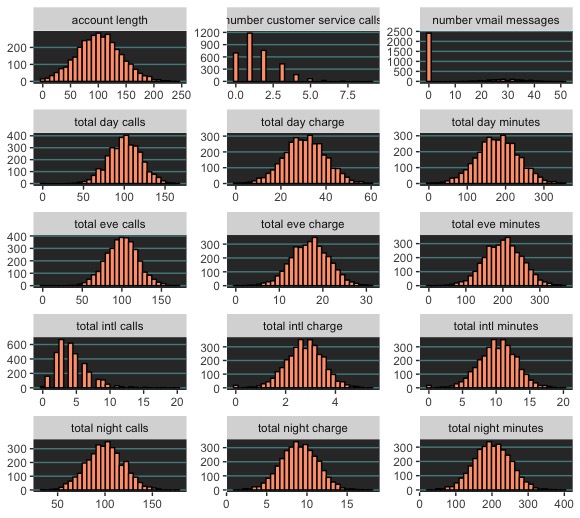
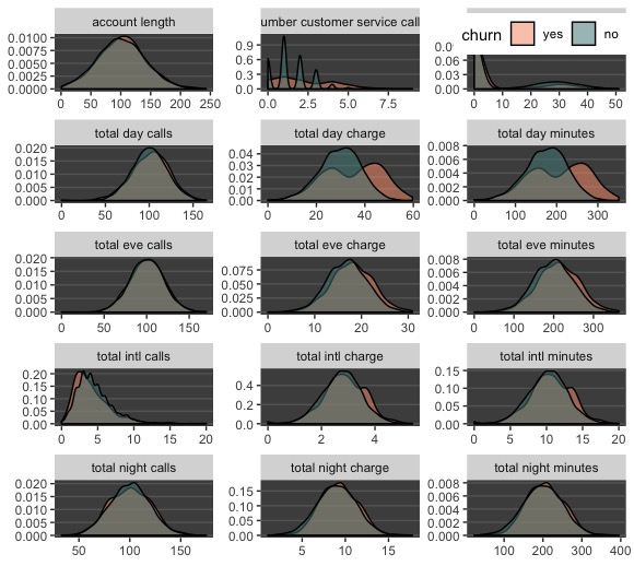
Exploring Numeric Data

The data were mostly well-behaved. However, notice on the left panel the column “number vmail messages”, which shows that most customers don’t have any. As far as how distributions differ for different churn outcomes, the density plot (pictured right) shows that churn and non-churn customers have similar distributions across the numeric variables. However, in the case of “total day charge” and “total day minutes”, churners make longer calls and rack up higher phone bills than non-churners do. This is useful information.

   

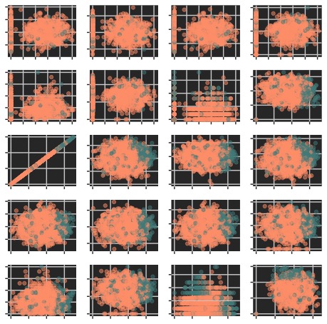
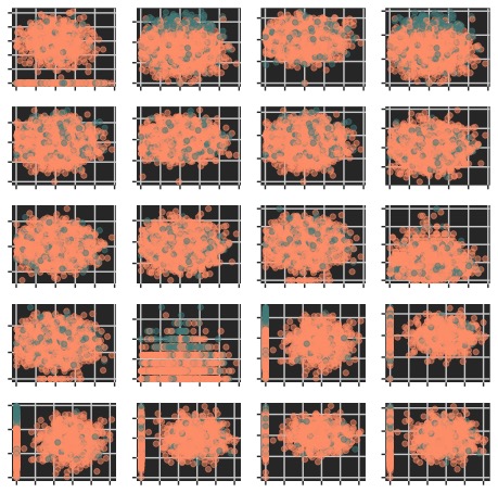
For the purpose of showing more about the numeric variable relationships, here are two (out of four) panels of scatterplots. Mainly we can see that churn and non-churn outcomes don’t appear to be linearly separable. Despite there being some clustering in a few of the variables, most of the churn and non-churn cases overlap. which suggests that linear classifier models shouldn’t be considered for use in predicting churn.

     

Exploring Categorical Data

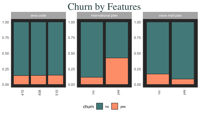
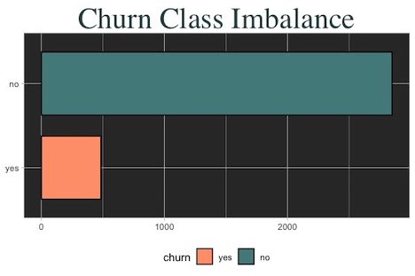
An important insight shown here is that nearly half of the customers on an international plan are ones who end up churning. This is even more extraordinary when we consider the severe disproportion between the two classes of customers ( shown below) – Despite being greatly outnumbered, “churners” make up a significant portion of customers on an international plan. In a similar (but lesser) light, customers that churn are more likely to not be on a voice mail plan than on one. Area code has no connection with churn.

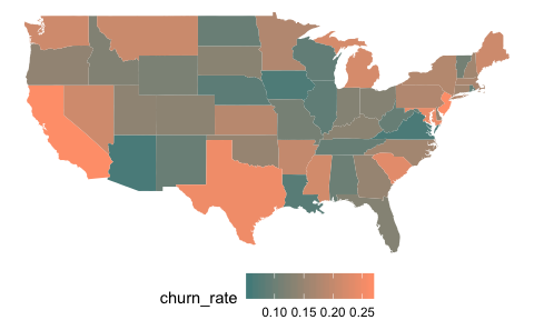
State demographics don’t indicate any clear pattern for churn rates. (below)

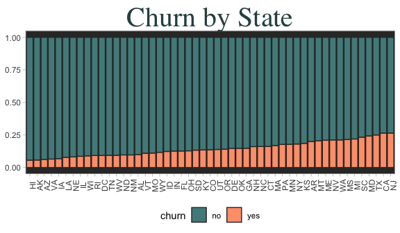
Churn and non-churn rates mapped to states also does not reveal any striking information, save for that three of the largest states do seem to have more churn.

Exploratory Findings

1.) Continuous predictors don’t appear linearly separable, so linear models won’t be considered for modeling.
2.) International plan and voice mail seem informative, as does total day charges. Perhaps a few states with super high or low churn rates will be informative in a model.
3.) There’s severe class imbalance in churn outcome which may pose challenges. This means that our model can achieve high accuracy just by guessing “no” for churn in every case. Therefore our model’s goal should not be overall accuracy, but instead aim at identifying cases of “churn = yes” (sensitivity).

Modeling

Only non-linear models (mostly tree-based) were used in this project. The training data was made into two versions, one using the regular set of variables, and another using an “expanded set” where categorical variables were coded into binary (1-0) values. The models used were K-Nearest-Neighbors, C50, Random Forest, and Gradient Boosted Machine.

K Nearest Neighbors The best fit had a sensitivity of .23, specificity of .97, and ROC of .66. The best fit chose a parameter of K = 5. Since sensitivity was so low, it is clear that KNN was unable to effectively identify customers that will churn.

C50 The optimal model achieved a sensitivity of .75, a specificity of .98, and ROC of .90. It used the expanded predictor set, and chose a “rules” model with no winnow.

Random Forest Sensitivity was .735, specificity was .987, and ROC was .90. The optimal Random Forest model used the expanded training set, choosing a parameter of “mtry” = 41.

Gradient Boosted GBM trained with the expanded predictor set achieved a sensitivity of .735. Optimal tuning parameters were: 1000 trees, interaction.depth = 5, shrinkage = 0.1, and n.minobsinnode = 10.

Model Test Performance

The model performances on the holdout testing data were very similar to their cross validated training performances.

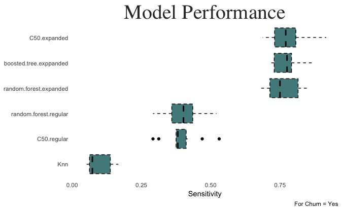
For the holdout test data, the C50 model built on the expanded dataset achieved the highest sensitivity value at .741. This performance was consistent with its training performance.

Further Model Improvements

There are further methods that can be used to improve our ability to predict churn accurately. When dealing with class imbalance, a classification model can be improved by changing the probability threshold of the prediction. Think of this as lowering the bar for the “evidence needed” to make a prediction – instead of determining a probability of 0.5 or higher as “yes”, we might broaden the decision range to 0.3 and higher to capture more values (and incur a certain amount of error as a tradeoff).

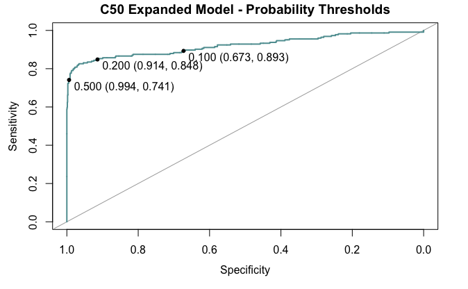
Pictured above, changing the decision threshold to a lower value such as .2 will presumably raise the C50 model’s sensitivity from .74 to .84, at little cost to specificity. Going beyond this point gives little raise to sensitivity and incurs a lot of false positives thereafter. Ideally, to alter the decision threshold would require testing on more data in order to be confident that this method is improving our ability to predict churn. Since there is no other data for testing, here it is safer not to alter the decision threshold.

Conclusion

The best models are the C50 and Random Forest models built on the expanded set of predictors. The most optimal model for predicting “churn = yes” correctly was the C50 model trained on the expanded training set. With a sensitivity of .74, it will correctly identify 74% of the customers that will churn. The model’s performance in terms of sensitivity can be further improved by altering the decision threshold cutoffs. However, without more data to test on, doing so would potentially result in bias.