Today I want to predict churn using data from a hypothetical telecom company. Although it isn’t real life data, it is based on real life data. The data are spread across 19 columns — 14 continuous, 4 categorical, and the outcome variable for prediction - “churn”. The dataset is small, with 3333 rows for training and 1667 for testing.
Before modeling, I need to explore the data structure – the distributions, class balances/imbalances, relationships between variables, etc. Are there any visual patterns in the data? How does churn relate to the continuous and discrete variables? These are questions I am asking at this initial stage. Let’s start with a series of histograms.
Data Overview
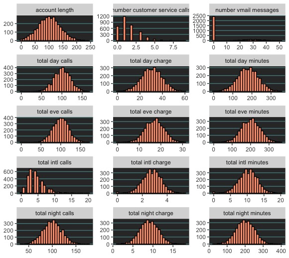
Most continuous predictors appear normally distributed. However, there are some exceptions “Customer service calls” and “total international calls” are somewhat right skewed, and the majority of values for “numer of mail messages” are all “0”, meaning it is probably a zero variance predictor. For the most part, these data are well behaved.
Let’s examine how these same predictors relate to churn. A density plot showing the variables’ distributions by class will suffice.
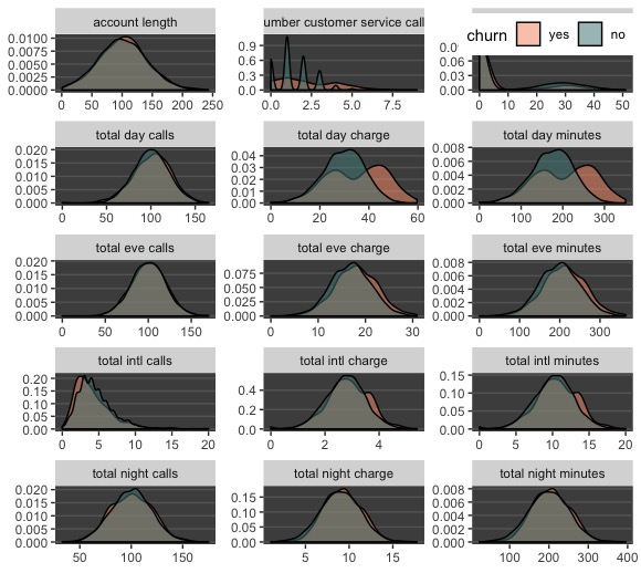
This density plot shows that “positive” churn has symmetrical distributions with that of the non-churners for most numeric predictors. (Note this is a density plot, so it depicts proportions, not quantities, of each class across a range of values.) We only see separation between red and green in amount of minutes per day and day charges, but these two variables clearly repeat the same information. One should probably be removed. Let’s continue by looking at how churn relates to the categorical variables.
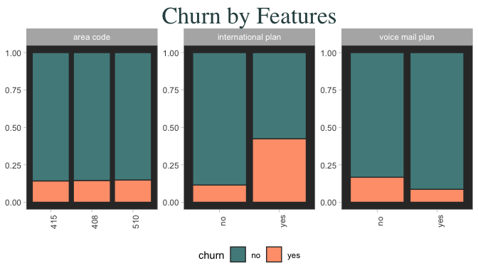
Categorical predictors are informative – Look at how many customers on an international plan end up churning! On the flipside, notice how churn outcome is unrelated to area code, but somewhat related to if they have voice mail. International plan and voice mail look like they will be useful predictors. Is “state” information useful at all?
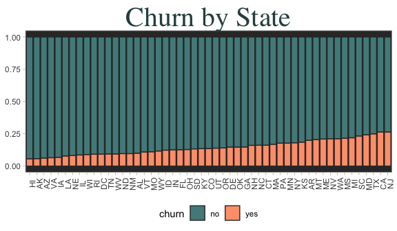
State information sure doesn’t look useful. From just looking at totals, it’s hard to see any kind of pattern. Also there doesn’t seem to be any interesting variation, even if we randomly scrambled them all. Another way to see if there is a here is to plot the churn data on a choropleth (a shaded map) plot.
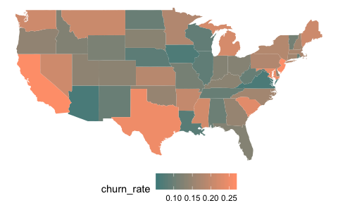
I still cannot determine any visual pattern for churn amongst states. This variable probably won’t be useful for most models. We can also check if there are obvious patterns between the continuous variables. Usually a panel of scatterplots can be made using pairs()' or 'GGally::ggpairs(). However, these functions dont work out of the box due to having too many variables.
With a bit of coding I aggregate the scatterplots into panels of 30, and produce a total of 4 grids like the two below. No need to clog up the page with all of them, most show a little clustering in some variables regarding the yes/no churn outcomes, and 1 or 2 instances of collinearity.
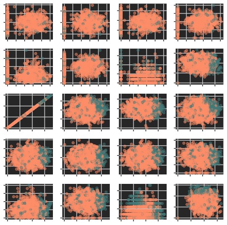
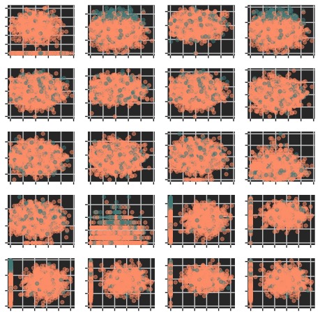
Clearly, Churn doesn’t appear to be linearly separable, meaning a linear classifier might not suffice. However, there does appear to be some clusering for some of these scatterplots. Still, tree models and KNN might perform better. My last check is to look at class balance for the outcome variable.
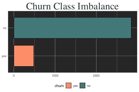
Churn classes are very imbalanced. Normally this can be fixed through up/down sampling the data, but here the training set has already been provided. Resampling here would bias predictions, so I’ll just bite the bullet.
Before modelling, let’s recap:
- Most continuous variables are evenly distributed.
- Continuous predictors do not appear linearly seprable on the face of things, but there is some clustering.
- There’s class imbalance in the outcome variable
churn. - International plan and voice mail seem informative, as does total day charges. Perhaps a few states with super high or low vlues will be informarive in a model that uses an expanded predictor set.
Now lets try to build some models to help predict churn I’ll use two versions of predictor sets to fit models, one with the regular set of variables, and another with an “expanded set” where categorical variables are coded into binary (1-0) values.
Modelling
Since data didn’t show linearity, I’ll start with a K Nearest Neighbors. Data needs to be numeric (so for classification, I’ll use binary values for all categorical variables) and data need to be preprocessed with scaling so that variables with higher values don’t outweigh the variables with lower values. The only tuning paramater is K, which will be automatically tuned across 20 values of tunelength.
##Expanded set
knn_expanded <- train(training_expanded, training_outcome, method = "knn", preProcess = c("center", "scale"),
                   trControl = ctrl, tuneLength = 20, metric = "Sens")
The optimal model has a paramater of K=5. ROC is .82, sensitivity .28, and specificty .98. Although ROC (area under the curve) is high, sensitivity is way too low. It seems we cannot effectively use KNN to identify customers that will churn.
Next let’s try a tree/rules model using C50. The model can fit both decision trees and rules based trees. It also has the option of “winnow” which means it prunes away predictors it deems less useful.
c50_regular <- train(training_regular, training_outcome, method = "C5.0", trControl = ctrl, tunegrid = expand.grid(trials = seq(25, 50, by = 2), model = c("tree", "rules"), winnow = c("TRUE", "FALSE")), metric = "Sens")

c50_expanded <- train(training_expanded, training_outcome, method = "C5.0", trControl = ctrl, tuneGrid = expand.grid(trials = seq(25, 50, by = 2), model = c("tree", "rules"), winnow = c("TRUE", "FALSE")), metric = "Sens")
Churn classes in this dataset are heavily imbalanced and that simply by predicting “No”, a model can achieve a high ROC like KNN did. What we want to maximize is sensitivity, and for that, the expanded C50 does a great job compared to the regular set. It fits a rules model with no winnow, and achieves a sensitivity value of .75, specificity of .98, and ROC of .909.
Next up, a random forest. Again, I’ll fit two models, using the normal set and the expanded set.
rf_regular <- train(training_regular, training_outcome, method = "rf", ntree = 1500, trControl = ctrl, tuneLength = 20, metric = "Sens", verbose = FALSE)


rf_expanded <- train(training_expanded, training_outcome, method = "rf", ntree = 1500, trControl = ctrl, tuneGrid = expand.grid(mtry = seq(25, 60, by = 2)), metric = "Sens", verbose = FALSE)
The optimal random forest model is the model using the expanded set, and it uses a paramater of mtry = 17. ROC is .89, sensitivity is .82, and specificity is .90. The quality of fit is good, but the model for the regular variable set performed worse.
Now let’s try a gradient boosted tree model.
gbm_regular <- train(training_regular, training_outcome, method = "gbm", trControl = ctrl, tuneLength = 20, metric = "Sens", tuneLength = 20 verbose = FALSE)

gbm_expanded <- train(training_expanded, training_outcome, method = "gbm", trControl = ctrl, tuneLength = 20, metric = "Sens")
Performance for the model trained on the expanded predictor set is slightly higher than the c50 model in terms of sensitivity. Let’s compare the sensitivity values of each model in a boxplot. Since the models were cross validated over 10 folds, we can be sure that these sensitivity estimates are stable.
Models built using the expanded predictor sets (categorical variables expanded into columns using hot coded binary values) performed much better than the models built on regular sets. Expanded random forest and c50 to be the best performers on the testing sets. Let’s see how they perform on hold out testing data.
## Use models to predict test data, evaluate performance.
knn_pred <- predict(knn_expanded, newdata = testing_expanded)
c50_normal_pred <- predict(c50_regular, newdata = testing_regular)
c50_expanded_pred <- predict(c50_expanded, newdata = testing_expanded)
rf_normal_pred <- predict(rf_regular, newdata = testing_regular)
## Make list of model predictions
models <- list("knn" = knn_pred, "c50" = c50_normal_pred, "c50 exp." = c50_expanded_pred, "random forest" = rf_normal_pred)

##Make list of all model predictions
predictions_list <- list("knn" = knn_pred, "c50_normal" = c50_normal_pred, "c50_expanded" = c50_expanded_pred)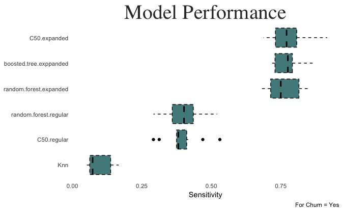
The c50 model built on the expanded dataset achieves the highest sensitivity, at .741.
There are a number of ways the sensitivity of these models could be improved. Sometimes resampling the data to balance the outcome variable can help. Also, setting a new probability threshold on the predictions would help if the class balance means there is a low signal for the class you’re trying to predict.
Say, instead of only predicting “Yes” if it has a probability of .5 or greater, we can lower the probability threshold of “evidence needed” to predict yes, to say .3, or .4, etc. Doing so will not change the model, but it will come at the cost of specificity. A rudimentary representation can be seen below, using the C50 model with the expanded predictor set.
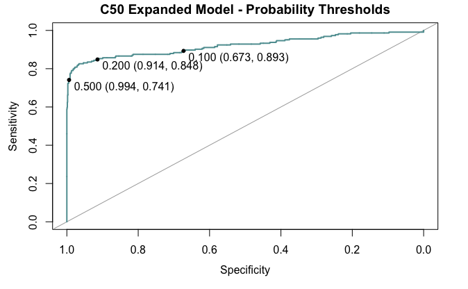
Above are probability thresholds set at .5, .2, and .1. Notice how sensitivity significantly improves if we determine a “yes” cutoff lower than .5, and that specificity isn’t impacted by this. However, when setting the threshold too low (.1), sensitivity tapers off, and comes with a much greater loss to specificity. At that point, half of our predictions would be false positives. Therefore setting a cutoff at around .2 or a bit more seems optimal. However, this is a hindsight bias and too risky to do if we dont have more data to test it on. Ideally we would an intial training set to compare models, another to tweak parameters and decision threholds, and a test set to test them all.
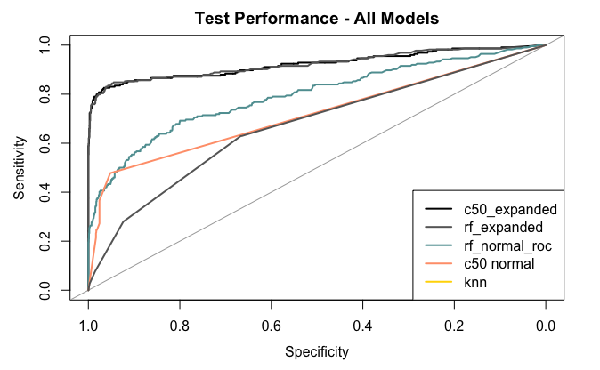
Let’s end by simply the test set performances of all models together.
Conclusion
The best models are the C50 and random forest models built on the expanded set of predictors. Since we are interested sensitivity (true positives for churn = “yes”), we can improve the performance of our predictions by altering the decision threshold cutoffs. But, since we do not have a separate training set of data to test the new cutoff on, doing so would create model bias. All in all, predicting churn was an informative exercise!
Note: If you wish to see code, feel free to check the code for this post on my github.