This is a continuation in my series of exploratory text analysis of 3 Chinese classic works. In the previous post, I calculated word counts for each book, and visualized common words using bar charts. This time, I’d like to examine word use across the texts with network visualization. The goal is to help see what’s common and what’s different between the texts regarding word usage.
Network visualization is particularly helpful for discovering simularities and differences between objects - this is because nodes and edges can form connections and clusters (or stay isolated). Thus, through a network structure we can get an idea of commonalities and differences between the word usages in these 3 works.
Disclaimer - the setup of this post is very similar to last time. I’m essentially importing the same data. So just skip past these first 2 code blocks.
library(tidyverse)
library(readr)
library(stringi)
library(tidygraph)
library(ggraph)


my_classics <- read_csv("~/Desktop/anything_data/content/post/my_classics.csv") %>%
  select(-1) %>%
  mutate(book = str_to_title(book))
simple_bigram <- function(x) {
if(length(x) < 2) {
return(NA)
} else {
output_length <- length(x) - 1
output <- vector(length = output_length)
for(i in 1:output_length) {
output[i] <- paste(x[i], x[i+1], sep = " ")
}
output
}
}
tokenizer <- function(text) {
unlist(lapply(stringi::stri_split_boundaries(text), function(x) simple_bigram(x)))
}
library(tmcn)
stopwordsCN <- data.frame(word = c(tmcn::stopwordsCN(),
"子曰", "曰", "於", "則","吾", "子", "不", "無", "斯","與", "為", "必",
"使", "非","天下", "以為","上", "下", "人", "天", "不可", "謂", "是以",
"而不", "皆", "不亦", "乎", "之", "而", "者", "本", "與", "吾", "則",
"以", "其", "為", "不以", "不可", "也", "矣", "子", "由", "子曰", "曰",
"非其", "於", "不能", "如", "斯", "然", "君", "亦", "言", "聞", "今",
"君", "不知", "无"))
##High frequency single-words by chapter
chapter_words <- my_classics %>%
mutate(word = map(word, function(x) unlist(stringi::stri_split_boundaries(x)))) %>%
unnest(word) %>%
mutate(word = str_replace_all(word, "[「」《》『』,,、。;:?!]", "")) %>%
filter(!is.na(word), !grepl("Invald", word)) %>%
anti_join(stopwordsCN) %>%
select(word, book, chapter_number) %>%
count(book, chapter_number, word) %>%
group_by(book, chapter_number) %>%
mutate(frequency = n/sum(n), book_edges = book) %>%
filter(frequency > .01) %>% ungroup() %>%
select(word, book, n, frequency, book_edges)
book_words <- my_classics %>%
mutate(word = map(word, function(x) unlist(stringi::stri_split_boundaries(x)))) %>%
unnest(word) %>%
mutate(word = str_replace_all(word, "[「」《》『』,,、。;:?!]", "")) %>%
filter(!is.na(word), !grepl("Invald", word)) %>%
anti_join(stopwordsCN) %>%
select(word, book) %>%
count(book, word) %>%
group_by(book) %>%
mutate(frequency = n/sum(n), book_edges = book) %>%
filter(frequency > .001) Plotting the edges in “arcs” helps avoid any overplotting or tangling that might exist in the case of too much interconnectivity, as we will soon see.
I’ve got 2 different ways of visualizing networks using words in these texts. First, let’s look at single word use between each text, one plot showing common words by each chapter/book, another by book.
Unfortunatly the blog squishes the plot a bit, so you might want to zoom in on it.
##Single Words by Chapter and Book
knitr::opts_chunk$set(fig.width=16, fig.height=12)

as_tbl_graph(chapter_words, directed = FALSE) %>% ggraph(layout = "fr") +
  geom_edge_arc(aes(edge_width = frequency, color = factor(book_edges), alpha = frequency)) +
  geom_node_point(color = "black", alpha = .65, size = 7, show.legend = FALSE) +
  geom_node_text(aes(label = name), color = "white",
                 family = "HiraKakuProN-W3", check_overlap = TRUE) +
  scale_edge_colour_manual(values = c("#b20047", "#00b274", "#FFB52A")) +
  theme(axis.text.x = element_blank()) +
  theme(axis.text.y = element_blank()) +
  theme(panel.background = element_rect(fill = "#cddbda"),
        plot.background = element_rect(fill = "#cddbda"),
        panel.grid.major = element_blank(), panel.grid.minor = element_blank(),
        plot.margin = margin(0, 0, 0, 0, "cm")) +
  guides(edge_width=FALSE, edge_alpha = FALSE) +
  labs(x = NULL, y = NULL,
       title = "\nCommon Characters\n in the Analects, Mozi, and Zhuangzi\n") +
  theme(plot.title = element_text(size = 25, vjust = -10, hjust = 0.5,
                                  family = "Palatino", face = "bold.italic",
                                  color = "#3d4040")) +
  theme(legend.position = "bottom", legend.title = element_blank(),
        legend.key = element_rect(color = "#454444", fill = "#f5fffe"),
        legend.text = element_text(size = 12, color = "#3d4040", family = "Palatino"),
        legend.key.width = unit(4, "line"),
        legend.background = element_rect(fill = "#cddbda"))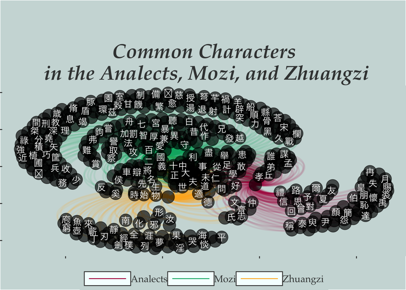
Compared to the above, doing the frequency counting by book seems to yeild a bit more balanced results. Of course frequency values become much lower that way, here I filter for greater than .001.
Single Words by Book
as_tbl_graph(book_words, directed = FALSE) %>%
ggraph(layout = "fr") +
geom_edge_arc(aes(edge_width = frequency, color = factor(book_edges), alpha = frequency)) +
geom_node_point(color = "black", alpha = .65, size = 7, show.legend = FALSE) +
geom_node_text(aes(label = name), color = "white",
family = "HiraKakuProN-W3", check_overlap = TRUE) +
scale_edge_colour_manual(values = c("#b20047", "#00b274", "#FFB52A")) +
theme(axis.text.x = element_blank()) +
theme(axis.text.y = element_blank()) +
theme(panel.background = element_rect(fill = "#cddbda"),
plot.background = element_rect(fill = "#cddbda"),
panel.grid.major = element_blank(), panel.grid.minor = element_blank(),
plot.margin = margin(0, 0, 0, 0, "cm")) +
guides(edge_width=FALSE, edge_alpha = FALSE) +
labs(x = NULL, y = NULL,
title = "\nCommon Characters\n in the Analects, Mozi, and Zhuangzi\n", caption = "Per Book, Frequency > .001") +
theme(plot.title = element_text(size = 25, vjust = -10, hjust = 0.5,
family = "Palatino", face = "bold.italic",
color = "#3d4040")) +
theme(legend.position = "bottom", legend.title = element_blank(),
legend.key = element_rect(color = "#454444", fill = "#f5fffe"),
legend.text = element_text(size = 12, color = "#3d4040", family = "Palatino"),
legend.key.width = unit(4, "line"),
legend.background = element_rect(fill = "#cddbda"))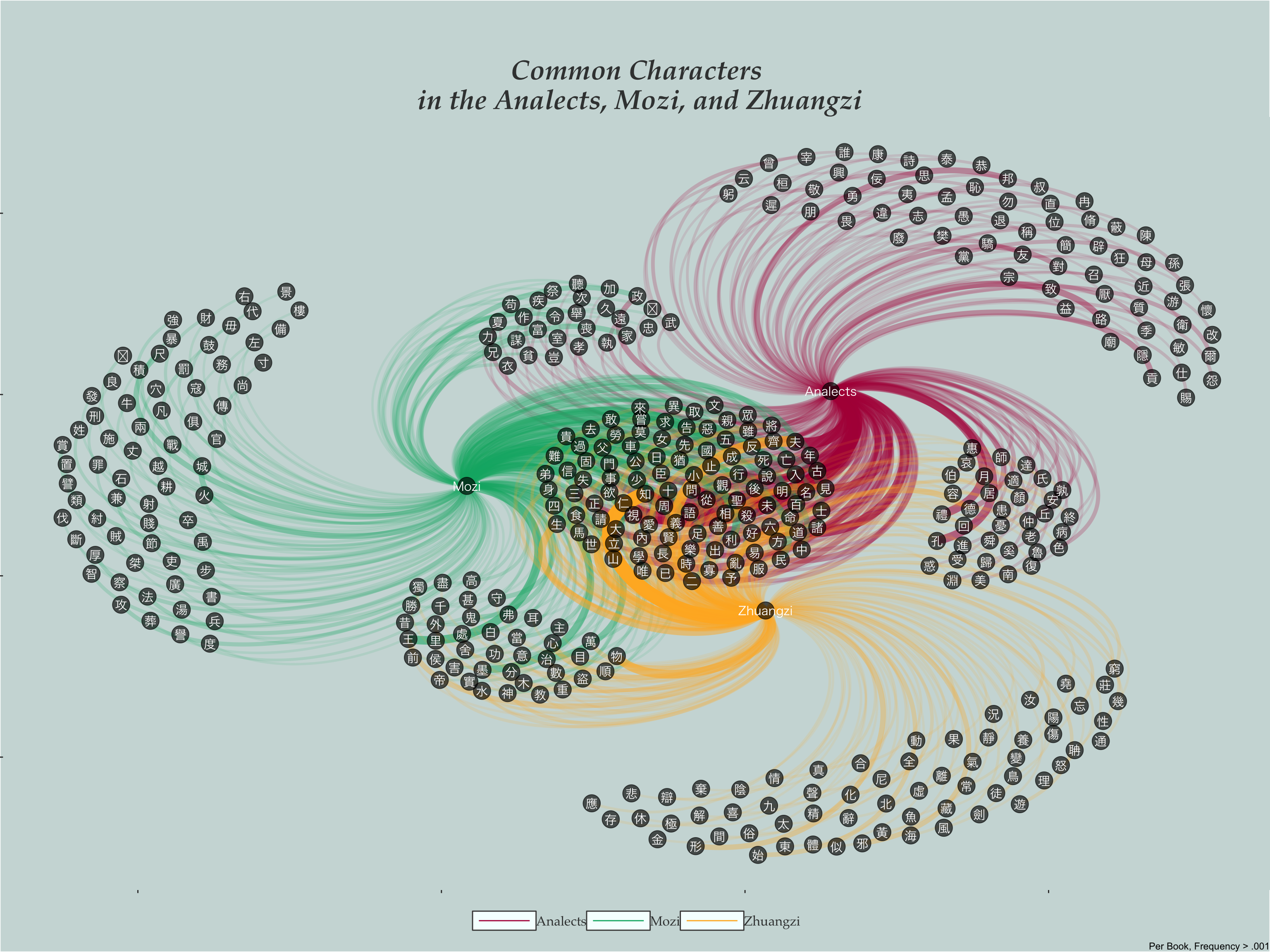 Regardless of calculating frequency by chapter and book or just by book, there are plenty of words that fall in between texts.
I’m not sure how useful this method of examining “simularity” of word usage is analytically; however, I think it works in a sense. If not for an algorithm, then at least for our general understanding. However, I do suspect that this type of networking does play into clustering, and from the looks of the plots, I imagine that the LDA algorithm might run into confusion distinguishing the books/chapters later.
##Now let’s plot bigrams
Here, a bigram is essentially two connected nodes. The connections (edges) between them are colored according to the text they appear in. Again, its a bit subjective on whether to calculate the bigrams by book or by each chapter and book. Conventional wisdom tells me that doing the calculation per chapter makes more sense, however, the Zhuangzi suffers from this operation. (Perhaps it has a greater word diversity per chapter?) So I decide to plot both ways.
##Bigrams by Chapter and Book
knitr::opts_chunk$set(fig.width=6, fig.height=6, fig.pos = "center")
bigrams <- my_classics %>%
mutate(word = str_replace_all(word, "[「」《》『』,,、。;:?!]", "")) %>%
mutate(word = map(word, function(x) tokenizer(x))) %>%
unnest(word) %>%
filter(!is.na(word)) %>%
separate(word, into = c("word1", "word2")) %>%
filter(!word1 %in% stopwordsCN$word, !word2 %in% stopwordsCN$word) %>%
unite("word", c("word1", "word2"), sep = " ")
chapter_bigrams <- bigrams %>%
count(book, chapter_number, word) %>%
arrange(book, -n) %>%
group_by(book, chapter_number) %>%
mutate(frequency = n/sum(n)) %>%
ungroup() %>%
select(-chapter_number)
chapter_bigrams %>%
separate(word, into = c("word1", "word2")) %>%
select(word1, word2, n, frequency, book) %>%
filter(frequency >= .02) %>%
as_tbl_graph(directed = FALSE) %>%
ggraph(layout = "fr") +
geom_edge_density() +
geom_edge_arc(aes(color = book),
alpha = .70, arrow = arrow(length = unit(1.5, "mm")),
start_cap = circle(3, "mm"), end_cap = circle(3, "mm"), edge_width = .75) +
geom_node_point(size = 7, color = "black", alpha = .75) +
geom_node_text(aes(label = name), color = "grey", family = "HiraKakuProN-W3", check_overlap = TRUE) +
scale_edge_colour_manual(values = c("#b20047", "#00b274", "#fdff00"))+
theme(axis.text.x = element_blank()) +
theme(axis.text.y = element_blank()) +
theme(panel.background = element_rect(fill = "#8AE3C2"),
plot.background = element_rect(fill = "#8AE3C2"),
panel.grid.major = element_blank(), panel.grid.minor = element_blank(),
plot.margin = margin(0, 0, 0, 0, "cm")) +
guides(edge_width=FALSE) +
labs(x = NULL, y = NULL, title = "Bigrams in the Analects, Mozi, and Zhuangzi", caption = "Per chapter, Frequency > .02") +
theme(plot.title = element_text(size = 35, vjust = -10, hjust = 0.5,
family = "Palatino", face = "italic",
color = "black")) +
theme(legend.position = "bottom", legend.title = element_blank(),
legend.key = element_rect(color = "black", fill = "#8AE3C2"),
legend.text = element_text(size = 12, color = "black", family = "Palatino"),
legend.key.width = unit(4, "line"),
legend.background = element_rect(fill = "#8AE3C2"))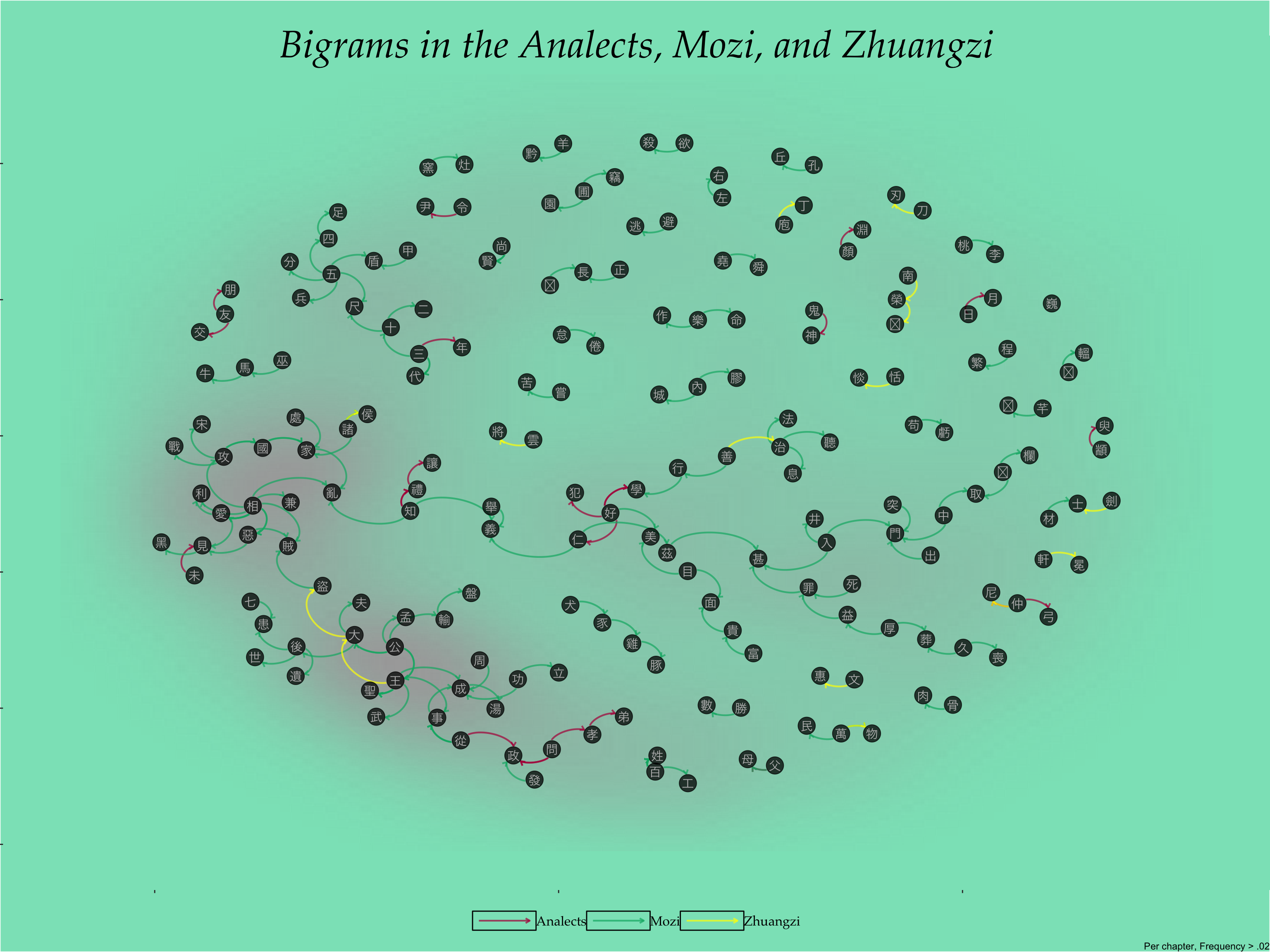 For the final plot, unfortunately many edges/links don’t show. Perhaps it is because many nodes are positioned so close together that the edges just aren’t drawn.
##Bigrams by Book
knitr::opts_chunk$set(fig.width=6, fig.height=6, fig.pos = "center")

book_bigrams <- bigrams %>%
  count(book, word) %>%
  arrange(book, -n) %>%
  group_by(book) %>%
  mutate(frequency = n/sum(n)) %>%
  ungroup()

book_bigrams %>%
  separate(word, into = c("word1", "word2")) %>%
  select(word1, word2, n, frequency, book) %>%
  filter(frequency >= .001) %>%
  as_tbl_graph(directed = FALSE) %>%
  ggraph(layout = "fr") +
  geom_edge_density() +
  geom_edge_arc(aes(color = book),
                alpha = .70, arrow = arrow(length = unit(1.5, "mm")),
                start_cap = circle(3, "mm"), end_cap = circle(3, "mm"), edge_width = .75) +
  geom_node_point(size = 7, color = "black", alpha = .75) +
  geom_node_text(aes(label = name), color = "grey", family = "HiraKakuProN-W3", check_overlap = TRUE) +
  scale_edge_colour_manual(values = c("#b20047", "#00b274", "#fdff00"))+
  theme(axis.text.x = element_blank()) +
  theme(axis.text.y = element_blank()) +
  theme(panel.background = element_rect(fill = "#8AE3C2"),
        plot.background = element_rect(fill = "#8AE3C2"),
        panel.grid.major = element_blank(), panel.grid.minor = element_blank(),
        plot.margin = margin(0, 0, 0, 0, "cm")) +
  guides(edge_width=FALSE) +
  labs(x = NULL, y = NULL, title = "Bigrams in\n the Analects, Mozi, and Zhuangzi", caption = "Per book, Frequency > .001") +
  theme(plot.title = element_text(size = 25, vjust = -10, hjust = 0.5,
                                  family = "Palatino", face = "italic",
                                  color = "black")) +
  theme(legend.position = "bottom", legend.title = element_blank(),
        legend.key = element_rect(color = "black", fill = "#8AE3C2"),
        legend.text = element_text(size = 12, color = "black", family = "Palatino"),
        legend.key.width = unit(4, "line"),
        legend.background = element_rect(fill = "#8AE3C2"))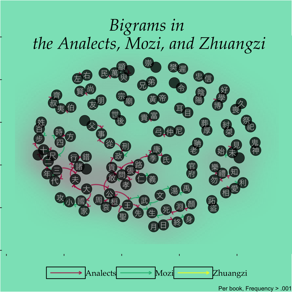
There we have it, two different network plots of words used in these 3 classic works. In the case of the single characters, there is a lot of commonality (as expected). In the case of the bigrams, there is a lot less in common between the works.
Before I close, I’d like to comment briefly on the tidygraph package which made these plots possible. Previously, I used igraph and found it powerful and quite robust, yet not too intuitive or user-friendly. Tidygraph changes all of that and allows network data to be manipulated in a way similar to the tidyverse methodology. I love tidygraph!
I hope you enjoyed these two network plots. Until next time!